Basis Splines

Overview

B-splines are commonly used as basis functions to fit smoothing curves to large data sets. To do this, the abscissa axis is broken up into some number of intervals, where the endpoints of each interval are called “breakpoints”. These breakpoints are then converted to “knots” by imposing various continuity and smoothness conditions at each interface. Given a nondecreasing knot vector t = {t₀, t₁, ..., t_n+k-1}, the n basis splines of order k are defined by

\[\begin{split}\begin{array}{ll} B_{i,1}(x) = & \left\{ \begin{array}{rl} 1 & \qquad t_i \le x < t_{i+1} \\ 0 & \qquad \textrm{else} \end{array} \right. \\ B_{i,k}(x) = & \dfrac{x - t_i}{t_{i+k-1} - t_i} B_{i,k-1}(x) + \dfrac{t_{i+k} - x}{t_{i+k} - t_{i+1}} B_{i+1,k-1}(x) \end{array}\end{split}\]

for i = 0, ..., n-1. The common case of cubic B-splines is given by k = 4. The above recurrence relation can be evaluated in a numerically stable way by the de Boor algorithm.

If we define appropriate knots on an interval [a,b] then the B-spline basis functions form a complete set on that interval. Therefore we can expand a smoothing function as

\[f(x) = \sum_i c_i B_{i,k}(x)\]

given enough \((x_j, f(x_j))\) data pairs. The coefficients c_i can be readily obtained from a least-squares fit.

B-Splines functions

bspline(a, b, N[, order])

bspline(knots[, order])

Create an object of type BSpline. In the first form it will create a basis splines in the interval from a to b with N uniformly spaced breaks. The order is 4 if unspecified, it corresponds to cubic splines. In the second form you should provide a non-decreasing list knots with all the points.

class BSpline

This is the class use to calculate the Basis Splines.

eval(x)

Return a column matrix with nbreak + order - 2 elements that stores the value of all the B-spline basis functions at the position x.

model(x)

Takes a column matrix of dimension N and returns a matrix of M columns and N rows where M = nbreak + order - 1. The matrix will contain, for each column, the value of the corresponding basis function evaluated in all the N position given by x.

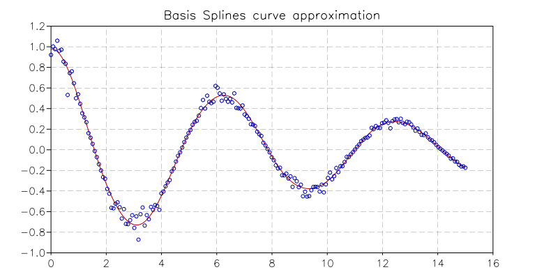
B-splines Example

The following example computes a linear least squares fit to data using cubic B-spline basis functions with uniform breakpoints. The data is generated from the curve \(y(x) = \cos(x) \exp(-x/10)\) on the interval [0,15] with Gaussian noise added:

matrix = require("lgsl.matrix")
bspline = require("lgsl.bspline")
rng = require("lgsl.rng")
rnd = require("lgsl.rnd")
linfit = require("lgsl.linfit")

-- number of points and breakpoints
n, br = 200, 10

f = function(x) return math.cos(x) * math.exp(-0.1 * x) end
xsmp = function(i) return 15 * (i-1) / (n-1) end

-- we calculate the simulated data
x, y = matrix.new(n, 1, xsmp), matrix.new(n, 1, function(i) return f(xsmp(i)) end)

-- we add a Gaussian noise and calculate weights
r = rng.new()
w = matrix.new(n, 1)
for i=1,n do
   local sigma = 0.1 * y[i]
   y:set(i,1, y[i] + rnd.gaussian(r, sigma))
   w:set(i,1, 1/sigma^2)
end

-- we create a bspline object and we calculate the model matrix X
b = bspline(0, 15, br)
X = b:model(x)

-- linear least-squares fit
c, cov = linfit(X, y, w)

-- plot; requires graph-toolkit.
graph = require("graph")

p = graph.plot('B-splines curve approximation')
p:addline(graph.xyline(x, X * c))
p:addline(graph.xyline(x, y), 'blue', {{'marker', size=5}})
p:show()

And the resulting plot is: