LGSL introduction

LGSL offers an intuitive interface to the numerical routines of the GNU Scientific Library (GSL) using Lua, an easy to learn and powerful programming languages. LGSL is based on the numerical modules of GSL Shell, and requires LuaJIT.

With LGSL, you can access the functions provided by the GSL library with great ease, without the need to write and compile a stand-alone C application. In addition, the power and expressiveness of the Lua language enables you to develop and test complex procedures to process your data and effectively use the GSL routines. LGSL combines usability with speed, as LuaJIT provides excellent execution speed that can be very competitive with compiled C or C++ code.

It is recommended to install the powerful graph-toolkit Lua module for creating plots.

To access a function from LGSL, you can either require the specific module lgsl.modulename:

m = require("lgsl.matrix")
A = m.new(2,2)

Alternatively, you can load the entire lgsl parent module, in which all modules are loaded by default:

lgsl = require("lgsl")

-- access functions directly from lgsl
B = lgsl.matrix.new(2,2)

-- list all loaded modules
for k,v in pairs(lgsl) do print(k) end

Note

In the examples in this manual, we do not use local variables. This allows all examples to be tried out in LuaJIT in interactive mode. However, in performance-critical situations, you are strongly encouraged to use local variables!

Real and complex numbers

In LuaJIT (or Lua 5.1), all numbers are internally stored in double precision; in this manual, we refer to this kind of number as a real number, as opposed to a complex number. LuaJIT does not have a distinct type to represent integer numbers; in other words, integer numbers are treated just like real numbers with all the implications that follow.

When you need to define a complex number you can use a native syntax like in the following example:

x = 3 + 4i

The rule is that when you write a number followed by an ‘i’ it will be considered as a pure imaginary number. The imaginary number will be accepted only if the ‘i’ follows immediately the number without any interleaving spaces. Note also that if you write ‘i’ alone this will be not interpreted as the imaginary unit but as the variable ‘i’. The imaginary unit can be declared by writing ‘1i’, because the ‘1’ at the beginning forces the interpreter to consider it as a number.

All the functions in math such as exp, sin, cos etc. work on real numbers. If you want to operate on complex numbers, you should use the functions defined in the complex module.

Matrices

The other important mathematical types in LGSL are matrices, either of complex or real numbers. In addition, Lua offers a native type called “table”. The latter is very useful for general purpose programming because it can store any kind of data or structures. However, you should be careful to not confuse Lua tables with matrices. You can work with both types as far as you understand the difference and use the appropriate functions to operate on them.

Most of the LGSL functions operate on real or complex matrices because of the nature of the GSL library itself.

Creating matrices

In order to define a matrix you have basically two options: you can enumerate all the values or you can provide a function that generates the terms of the matrix. In the first case you, should use the matrix.def() like in the following example:

matrix = require("lgsl.matrix")
th = math.pi/8 -- define the angle "th"

-- define 2x2 rotation matrix for the given angle "th"
m = matrix.def {{math.cos(th), math.sin(th)}, {-math.sin(th), math.cos(th)}}

You can remark that we have used the matrix.def() function without parentheses to enclose its arguments. The reason is that, when a function is called with a single argument which is a literal table or string, you can omit the enclosing parentheses. In this case we have therefore omitted the parentheses because matrix.def() has a single argument that is a literal table.

As a general remark, in performance-sensitive situations, it may be useful to store functions such as math.sin() and math.cos() in local variables sin and cos instead of accessing the math library every time.

You can also define a column matrix using the function matrix.vec() as follows:

v = matrix.vec {math.cos(th), math.sin(th)}

The other way to define a matrix is through the matrix.new() function (or matrix.cnew() to create a complex matrix). This function takes the number of rows and columns as the first two arguments and a function as an optional third argument. Let us see an example to illustrate how it works:

-- define a matrix whose (i, j) element is 1/(i + j)
m = matrix.new(4, 4, function(i,j) return 1/(i + j) end)`

The function passed to matrix.new() takes two arguments, respectively the row and column number, and returns the value that should be assigned to the corresponding matrix element. Of course, you are not forced to define the function in the same line; you can define it before and use it later with the matrix.new() function as in the following example:

sf = require("lgsl.sf")

-- define the binomial function
function binomial(n, k)
  if k <= n then
      return sf.choose(n-1, k-1)
  else
      return 0
  end
end

-- define a matrix based on the function just defined
m = matrix.new(8, 8, binomial)

This is the result:

>>> print(m)
[  1  0  0  0  0  0  0  0 ]
[  1  1  0  0  0  0  0  0 ]
[  1  2  1  0  0  0  0  0 ]
[  1  3  3  1  0  0  0  0 ]
[  1  4  6  4  1  0  0  0 ]
[  1  5 10 10  5  1  0  0 ]
[  1  6 15 20 15  6  1  0 ]
[  1  7 21 35 35 21  7  1 ]

An alternative compact writing could have been:

m = matrix.new(8, 8, function(n,k) return k <= n and sf.choose(n-1, k-1) or 0 end)

where we have again used the short function notation and the Lua logical operators and and or.

Matrix operations

If we want to obtain the inverse of the matrix defined above we can use the function matrix.inv(). Let us see how it works by using the matrix m defined above and taking its inverse:

-- we define the matrix
m = matrix.new(8, 8, function(n,k) return k <= n and sf.choose(n-1, k-1) or 0 end)

-- we obtain the inverse
minv = matrix.inv(m)

Then the matrix minv will be equal to:

>>> =minv
[   1   0   0   0   0   0   0   0 ]
[  -1   1   0   0   0   0   0   0 ]
[   1  -2   1   0   0   0   0   0 ]
[  -1   3  -3   1   0   0   0   0 ]
[   1  -4   6  -4   1   0   0   0 ]
[  -1   5 -10  10  -5   1   0   0 ]
[   1  -6  15 -20  15  -6   1   0 ]
[  -1   7 -21  35 -35  21  -7   1 ]

If we want to check that minv is actually the inverse of m, we can perform the matrix multiplication to check:

>>> =minv * m
[ 1 0 0 0 0 0 0 0 ]
[ 0 1 0 0 0 0 0 0 ]
[ 0 0 1 0 0 0 0 0 ]
[ 0 0 0 1 0 0 0 0 ]
[ 0 0 0 0 1 0 0 0 ]
[ 0 0 0 0 0 1 0 0 ]
[ 0 0 0 0 0 0 1 0 ]
[ 0 0 0 0 0 0 0 1 ]

and as we should expect, we have actually obtained the unit matrix.

The matrix inverse can be used to solve a linear system, so let us try that. First we define a column vector, for example:

b = matrix.new(8, 1, function(i) return math.sin(2*math.pi*(i-1)/8) end)
>>> =b
[           0 ]
[  0.70710678 ]
[           1 ]
[  0.70710678 ]
[           0 ]
[ -0.70710678 ]
[          -1 ]
[ -0.70710678 ]

The we can solve the linear system m * x = b using the inverse matrix minv as follows:

x = minv * b
>>> =x
[           0 ]
[  0.70710678 ]
[ -0.41421356 ]
[ -0.17157288 ]
[  0.34314575 ]
[ -0.10050506 ]
[ -0.14213562 ]
[  0.14213562 ]

so that the resulting column matrix x will satisfy the equation m * x = b.

The reader familiar with linear algebra computations may argue that using matrix inversion to solve a linear system is inefficient. This is actually true and LGSL offers the function matrix.solve() to solve a linear system efficiently. So in the example above we could have used the function matrix.solve() as follows:

x = matrix.solve(m, b)

to obtain the same result of above.

Working with complex matrices

In the example above we have shown how to solve a linear system in the form m * x = b. We may wonder how to manage the case when m or b are complex. The answer is easy, since LGSL always checks the type of the matrix, and the appropriate algorithm is selected.

So, to continue the example above, we can define b as a complex vector as follows:

b = matrix.cnew(8, 1, |i| complex.exp(2i*pi*(i-1)/8))
>>> =b
[                       1 ]
[  0.70710678+0.70710678i ]
[                       i ]
[ -0.70710678+0.70710678i ]
[                      -1 ]
[ -0.70710678-0.70710678i ]
[                      -i ]
[  0.70710678-0.70710678i ]

and then we can use the function matrix.solve() as above and we will obtain a complex matrix that solves the linear system.

Please note that above we have used the function matrix.cnew() to create a new complex matrix. The reason is that we need to inform LGSL in advance if we want a complex matrix.

In general, LGSL tries to ensure that all the common matrix operations transparently handle real or complex matrices.

Matrix indexing

When indexing the matrix, only one index is permitted, so the syntax m[2] is OK but m[2,3] will not be accepted. This is a limitation of the Lua programming language.

When you write m[2] you will obtain the second row of the matrix m but in column form. So, if we use the matrix m defined above we could have:

>>> m[5]
[ 1 ]
[ 4 ]
[ 6 ]
[ 4 ]
[ 1 ]
[ 0 ]
[ 0 ]
[ 0 ]

It may seem odd that the row is returned in column form but it is actually convenient because many functions accept a column matrix as input. The idea is that in LGSL, column matrices play the role of vectors.

Following the same logic as above, if you index a column matrix you will just obtain its n-th element (as returning a 1x1 matrix will be not very useful). So you can have for example:

>>> m[5][4]
4

At this point it should be clear that, in general, you can access the elements of a matrix with the double indexing syntax m[i][j].

Something that is important to know about the matrix indexing to obtain a row is that the column matrix refers to the same underlying data as the original matrix. As a consequence, any change to the elements of the derived matrix will also be effective for the original matrix.

The indexing method that we have explained above can be used not only for retrieving the matrix elements or an entire row, but it can be equally used for assignment. This means that you can use double indexing to change an element of a matrix. If you use single indexing, you can assign the content of a whole row all at once.

Note

Regarding efficiency: the double indexing method can be slow and should be probably avoided in a tight loop where the performance is important. In this case you should use the methods get() and set(). Another opportunity is to directly address matrix data by using its data field, but this requires particular attention since these kinds of operations are not safe and could easily crash the application.

You can find more details in the chapter about GSL FFI interface.

An Example

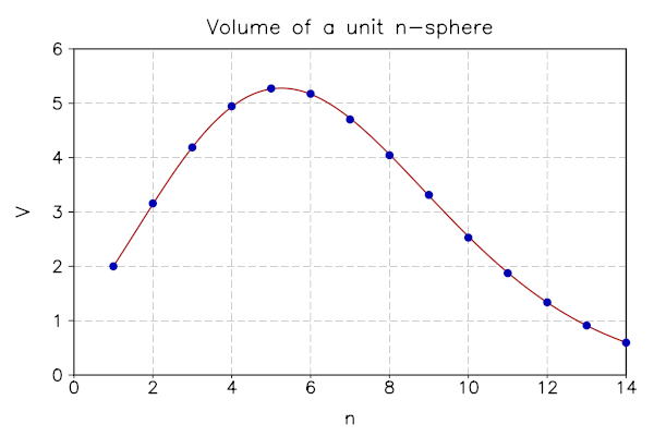
To illustrate most of the key features of LGSL, let us write a short script to calculate the volume of an n-dimensional unit sphere and compare it with the analytical solution of \(V_n=\pi^{n/2}/ \Gamma(1+n/2)\).

For the integration in high dimensions, we will use the Monte Carlo VEGAS implementation, that is included in LGSL.

You must require the necessary modules before you can use them:

vegas = require("lgsl.vegas")

sf = require("lgsl.sf") -- for the analytical solution, see below
iter = require("lgsl.iter") -- for defining the integration boundaries

Now we need to define the integrand function. Since we want to calculate the volume of an n-dimensional sphere, the function should accept an n-tuple of coordinates and return 1 if the sampling point is inside the unit sphere or 0 otherwise. To work correctly, the VEGAS algorithm assumes that the integrand function takes a single argument that is a table with the n coordinates. Since the computation depends on the dimension n of the space, we need to take this into account. The solution is to define a function that we can call getunitsphere, that returns the integrand function for the n-dimension space.

The n-dimensional integrand function itself calculates the summed square of the table values for a given size which equals \(R^2=\sum_{i=1}^nx_i^2\). So getunitsphere can be defined as follows:

function getunitsphere(n)
   return function(x)
      local s = 0
      for k= 1, n do s = s + x[k]^2 end
      return s < 1 and 1 or 0
   end
end

This is the function we will use to integrate later.

For visualising our results, we will use the graph module, which can be required as follows:

graph = require("graph")

Now we can prepare a graph path that will hold all calculated values (graph.path()):

ln = graph.path(1, 2) -- 1-sphere = [-1, 1] (length 2)

Now, we can start to calculate the volume of the unit sphere of the first 14 dimensions:

max_dim = 14
for d=2, max_dim do

   local a = iter.ilist(function() return 0 end, d)
   local b = iter.ilist(function() return 1 end, d)
   local calls, n = d*1e4,1

   -- Obtaining monte carlo vegas state object
   local s = vegas.integ(getunitsphere(d),a,b,calls)

   --Increasing the number of calls to reach a satisfying result
   while(s.sigma/s.result > 0.005) do
      s = s.continue(calls*(2^n))
      n=n+1
   end

   ln:line_to(d,s.result*2^d)
end

The loop consists of three major parts. In the first part, we initialize the important variables with the iter.ilist() function, which conveniently creates vectors of any size with a value provided by the function. In this case a and b contain the lower and the upper boundaries for the integration.

The Monte Carlo VEGAS integrator vegas.integ() derives the number of dimensions from the length of the bounds vector, #a. By calling vegas.integ() with the desired unitsphere function, an integrator is created for this number of dimensions, and the Monte Carlo VEGAS algorithm is being invoked. It returns a state table s with the result itself, the precision sigma, the number of iterations calls it took, and a continuation function continue that can be called to recalculate the result with higher precision.

Depending on the relative precision s.sigma/s.result, we continue to recalculate the integral with increasing numbers of iterations. When it is done, we add the dimension and the result to our given path by line_to().

We can now proceed to compare the data with analytical solutions and plot these results. First we need to initialize a graph.plot() object. Then we can add the data to the plot with add() and the result of the analytical solution with addline(). Note that you can change the appearance of the data points at this moment. We are going for markers with size 8. The plot is created as follows:

p = graph.plot('Volume of a unit n-sphere')
p.clip, p.pad = false, true
analytic = function(n)
  return math.pi^(n/2) / sf.gamma(1+n/2)
end
p:addline(graph.fxline(analytic, 1, max_dim))
p:add(ln, "blue", {{'marker', size=8}})
p.xtitle="n"
p.ytitle="V"
p:show()

Also note that we use sf.gamma() from the special functions section, which offers all such functions that you can find in the GSL library. After setting the axis-names with xtitle() and ytitle(), we are ready to show the plot with show():

Here is the code as a whole (which uses local variables):

local vegas = require("lgsl.vegas")
local sf = require("lgsl.sf") -- for the analytical solution, see below
local iter = require("lgsl.iter") -- for defining the integration boundaries

local function getunitsphere(n)
   return function(x)
      local s = 0
      for k= 1, n do s = s + x[k]^2 end
      return s < 1 and 1 or 0
   end
end

local graph = require("graph")
local ln = graph.path(1, 2) -- 1-sphere = [-1, 1] (length 2)
local max_dim = 14

--Calculating the volume of d-dimensional sphere
for d=2, max_dim do
   --Intializing work varaibles
   local a = iter.ilist(function() return 0 end, d)
   local b = iter.ilist(function() return 1 end, d)
   local calls, n = d*1e4,1

   --Obtaining monte carlo vegas callback
   local s = vegas.integ(getunitsphere(d),a,b,calls)
   local fmt = "Volume = %.3f +/- %.3f "
   print(string.format(fmt,s.result*2^d,s.sigma*2^d))

   --Increasing the number of calls to reach a satisfying result
   while(s.sigma/s.result > 0.005) do
      print("Increasing accuracy, doubling number of calls...")
      s = s.continue(calls*(2^n))
      print(string.format(fmt,s.result*2^d,s.sigma*2^d))
      n=n+1
   end
   ln:line_to(d,s.result*2^d)
end

--plotting a comparison of the numerical result with the analytical solution
local p = graph.plot('Volume of a unit n-sphere')
p.clip, p.pad = false, true
local analytic = function(n) 
  return math.pi^(n/2) / sf.gamma(1+n/2)
end
p:addline(graph.fxline(analytic, 1, max_dim))
p:add(ln, "blue", {{'marker', size=8}})
p.xtitle="n"
p.ytitle="V"
p:show()

This rather simple example showed quite a lot of important features of LGSL and graph-toolkit. Creating data structures with iterators is very common.

With the function getunitsphere(), we have shown that some problems can be solved in an elegant way by returning a function. These kinds of functions are called closures because they refer to local variables declared outside of the function body itself. In this particular case, the function returned by getunitsphere() is a closure because it refers to the variable n defined outside its body. The function s.continue() returned by vegas.integ() is also another example of closure since it refers to the current state of the VEGAS integration.