LGSL Examples

In this chapter we give some usage examples of LGSL.

Home-made Bessel Functions

The Bessel function \(J_n\) for integer values of n can be defined with the following integral:

\[J_n(x) = {1 \over \pi} \int_0^\pi \cos(n \tau - x \sin \tau) \textrm{d}\tau\]

We can use this definition to define our home-made Bessel function. To perform the integral we need to use the integ.integ() function and provide the function to integrate. This is easy like eating a piece of cake:

integ = require("lgsl.integ").integ
function bessJ(x, n)
   local epsabs, epsrel = 1e-8, 1e-4
   -- we define the function to integrate
   local f = function(t) return math.cos(n*t - x*math.sin(t)) end
   return 1/math.pi * integ(f, 0, math.pi, epsabs, epsrel)
end

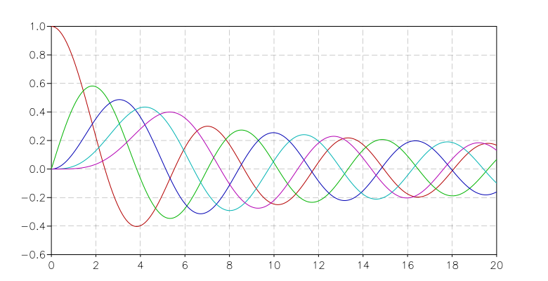
The definition of bessJ takes x and n as arguments and calculates the definite integral between 0 and \(\pi\). Using the graph module from the package graph-toolkit, we can plot the results for various values of n:

graph = require("graph")
p = graph.plot('Bessel Functions Jn, n=0 ... 5')
for n=0, 5 do
   p:addline(graph.fxline(function(x) return bessJ(x,n) end,  0, 20), graph.rainbow(n+1))
end
p:show()

to obtain the following result:

Then we can also calculate a matrix with the tabulated values. For example, we can use the columns of the matrix to span different values of n. We write:

matrix = require("lgsl.matrix")
m = matrix.new(200, 6, function(k,n) bessJ((k-1)/10, n-1) end)

And we obtain the following matrix:

[           1           0           0           0           0           0 ]
[    0.997502   0.0499375  0.00124896 2.08203e-05 2.60286e-07           0 ]
[    0.990025   0.0995008  0.00498335  0.00016625 4.15834e-06 8.31945e-08 ]
[    0.977626    0.148319   0.0111659 0.000559343  2.0999e-05 6.30443e-07 ]
[    0.960398    0.196027   0.0197347  0.00132005 6.61351e-05 2.64894e-06 ]
[     0.93847    0.242268    0.030604  0.00256373 0.000160736 8.05363e-06 ]
[    0.912005    0.286701   0.0436651  0.00439966  0.00033147 1.99482e-05 ]
[    0.881201    0.328996   0.0587869  0.00692965 0.000610097 4.28824e-05 ]
[    0.846287    0.368842   0.0758178   0.0102468  0.00103298 8.30836e-05 ]
[    0.807524     0.40595   0.0945863    0.014434  0.00164055 0.000148658 ]
[    0.765198    0.440051    0.114903   0.0195634  0.00247664 0.000249758 ]
[ ... ]

Zernike Polynomials

Taken from Wikipedia

In mathematics, the Zernike polynomials are a sequence of polynomials that are orthogonal on the unit disk. Named after Frits Zernike, they play an important role in beam optics.

Definitions

There are even and odd Zernike polynomials. The even ones are defined as

\[Z_n^m(\rho, \phi) = R_n^m(\rho) \cos(m \phi)\]

and the odd ones as

\[Z_n^{-m}(\rho, \phi) = R_n^m(\rho) \sin(m \phi)\]

where m and n are nonnegative integers with \(n \ge m\),:math:phi is the azimuthal angle, and \(\rho\) is the radial distance. The radial polynomials \(R_n^m\) are defined as

\[R_n^m(\rho) = \sum_{k=0}^{(n-m)/2} \frac{(-1)^k (n-k)!}{k! ((n+m)/2-k)! ((n-m)/2 - k)!} \rho^{n - 2 k}\]

for \(n - m\) even, and are identically 0 for \(n - m\) odd. For \(m = 0\), the even definition is used which reduces to \(R_n^0 (\rho)\).

Implementation

The above formula can be implemented quite straightforwardly in LGSL with only a subtle point about the factorials in the denominator. The problem is that in some cases you can have the factorial of a negative number and if you feed a negative number to the fact() function, you will get an error.

Actually the meaning of the formula is that the factorial of a negative number is \(\infty\) and so, since it appears in the denominator, its contribution to the sum is null. So, in order to implement this behavior we just define an auxiliary function that returns the inverse of the factorial and zero when the argument is negative.

So here is the code for the radial part:

fact = require("lgsl.sf").fact

-- inverse factorial function definition
invf = function(n)
  return n >= 0 and 1/fact(n) or 0
end

-- radial part of Zernike's polynomial
function zerR(n, m, p)
   local ip, im = (n+m)/2, (n-m)/2
   local z = 0
   for k=0, im do
      local f = fact(n-k) * (invf(k) * invf(ip-k) * invf(im-k))
      if f > 0 then z = z + (-1)^k * f * p^(n-2*k) end
   end
   return z
end

Next, we define Zernike’s function completed with the angular part:

function zernicke(n, m, p, phi, even)
   local pf = even and math.cos(m*phi) or math.sin(-m*phi)
   return zerR(n, m, p) * pf
end

Now we are ready to compute our function. The only missing piece is the relation between \(\rho\), \(\phi\) and the Cartesian coordinates but this is trivial:

\[\begin{split}\begin{array}{ll} \rho = & \sqrt{x^2 + y^2} \\ \phi = & \tan^{-1}(y, x) \end{array}\end{split}\]

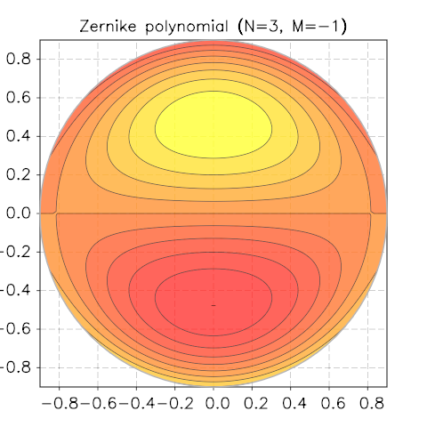
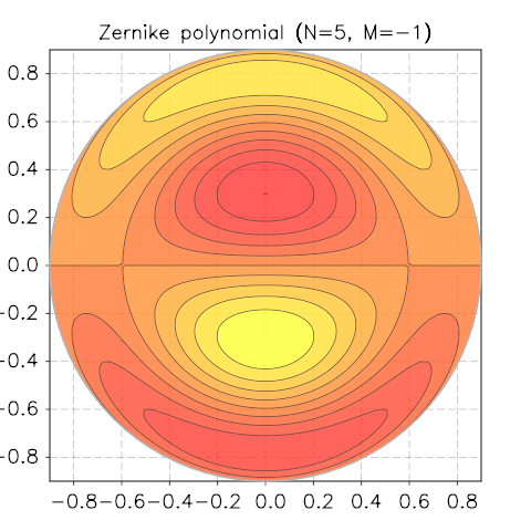
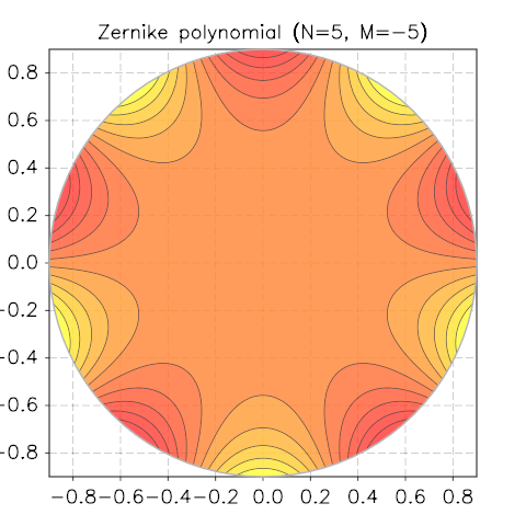
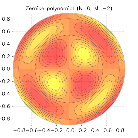
To visualise the functions, we will use the contour module of the graph-toolkit package. Let us define our sample function in terms of x and y and use it to call the function contour.polar_plot():

contour = require("graph.contour")
N, M = 8, -2
f = function(x,y) return zernicke(N, M, math.sqrt(x^2+y^2), math.atan2(y,x)) end
p = contour.polar_plot(f, 0.2, {gridx= 81, gridy= 81, levels= 10})
p.title = string.format('Zernike polynomial (N=%i, M=%i)', N, M)

We show a few screenshots of the contour plot for various N and M.